Velocity-time graphs are essential tools for understanding motion in physics....
Easy Guide: Find Acceleration and Distance on Velocity-Time Graphs for Kids
Z
Zoë@zoe_lewis
1
of 2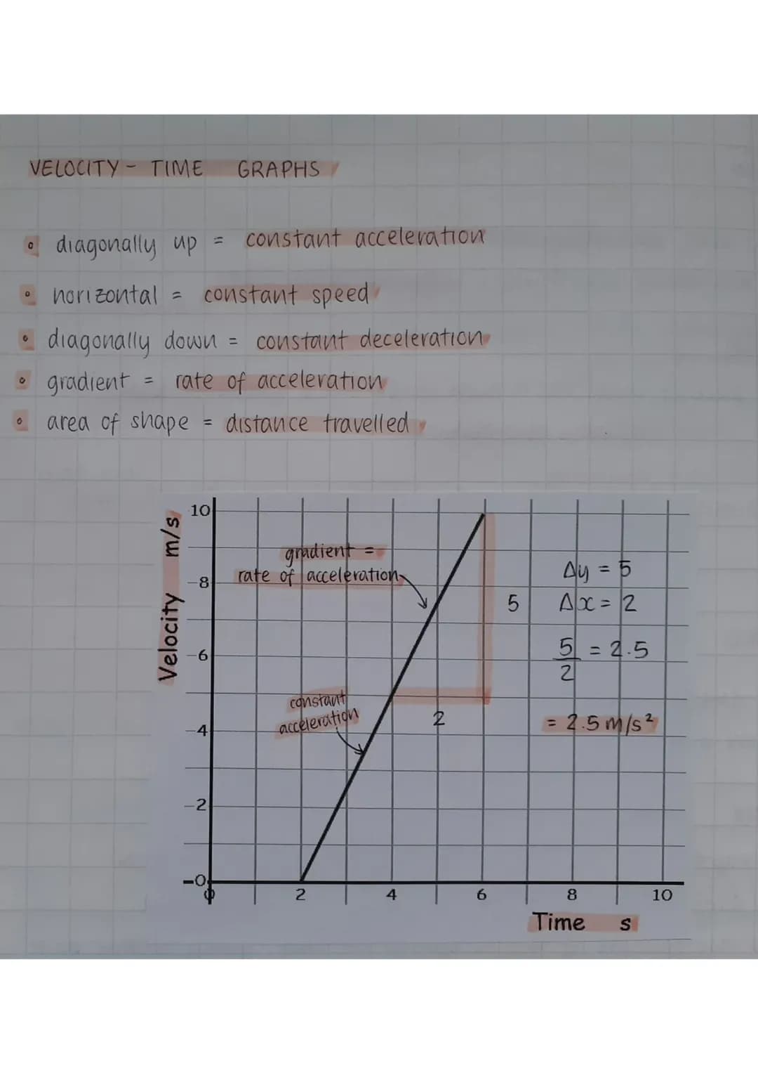
2
of 2
We thought you’d never ask...
What is the Knowunity AI companion?
Our AI Companion is a student-focused AI tool that offers more than just answers. Built on millions of Knowunity resources, it provides relevant information, personalised study plans, quizzes, and content directly in the chat, adapting to your individual learning journey.
Where can I download the Knowunity app?
You can download the app from Google Play Store and Apple App Store.
Is Knowunity really free of charge?
That's right! Enjoy free access to study content, connect with fellow students, and get instant help – all at your fingertips.
Similar content
Most popular content: Acceleration
1Most popular content in Maths
9Comprehensive Maths Concepts
Explore essential mathematical concepts including powers, geometry, statistics, and probability. This resource features 65 pages of detailed explanations, diagrams, and examples to enhance your understanding of topics such as right triangles, volume calculations, and data representation. Ideal for students seeking to strengthen their numeracy skills and grasp complex mathematical principles.
1080,0176,321
GCSE Maths (Higher) // Revision Guide
The only GCSE maths (higher) revision guide you need to get a grade 9! Contains every topic, each with all potential question types and their solutions.
102,56660
M
Medium Level alerbra
Master challenging maths concepts with this medium level flashcard set designed for grade 7/8 students. Strengthen your problem-solving skills and boost your confidence in maths!
78253
M
Mastering Maths: Essential Concepts for Grade 10
Boost your math skills with this comprehensive flashcard set covering key concepts for grade 10. Perfect for exam preparation and building a strong foundation in mathematics.
105401
Comprehensive Maths Concepts
Explore essential mathematical concepts including polynomial theorems, logarithmic properties, trigonometric functions, and integration techniques. This resource covers everything from solving inequalities to understanding exponential functions, providing a solid foundation for A-level mathematics. Ideal for students aiming for top grades.
1222,0161,817
M
Mastering Medium-Level Maths: Essential Flashcards for Grade 11 Students
Boost your Maths skills with this comprehensive set of flashcards designed specifically for Grade 11 students. Covering medium-level topics, these cards will help you ace your exams and build a solid foundation for advanced Maths.
119533
Comprehensive Maths Concepts
Explore essential higher mathematics concepts including calculus, trigonometry, polynomials, and vector analysis. This summary covers key topics such as differentiation, integration, quadratic equations, and the properties of circles, providing a solid foundation for exam preparation. Ideal for students seeking a concise yet thorough review of advanced mathematical principles.
S51,94157
M
maths SOHCAHTOA
Trigonometric ratios SOHCAHTOA for calculating angles and sides in right-angled triangles.
112200
P
Percentage,fractions and decimals
how well do you know percentages,fractions and decimals
73093
Most popular content
9Sociology of Education Overview
Explore comprehensive A-Level Sociology notes on the education system, covering key theories, policies, and sociological perspectives. This resource includes insights on marketisation, gender roles, cultural deprivation, and educational inequalities, providing a thorough understanding of how education shapes social stratification and individual achievement. Ideal for exam preparation and in-depth study.
12102,8353,040
Sociology of Families: Comprehensive Revision
Dive into an extensive overview of family dynamics, perspectives, and patterns in sociology. This resource covers key concepts such as family diversity, gender roles, marriage, and the impact of social policies on family structures. Perfect for A-Level Sociology students preparing for Paper 2.
1273,6032,306
Criminology: Crime & Punishment Overview
Comprehensive mindmaps covering key concepts in the Crime and Punishment topic for WJEC Criminology Unit 4. This resource includes detailed insights into the Criminal Justice System, crime prevention strategies, sentencing models, and the roles of various agencies. Ideal for A-Level revision, ensuring you grasp essential theories and legislative processes to excel in your exams.
1254,8581,059
Comprehensive Crime & Deviance Overview
Explore an extensive revision of crime and deviance topics, including theories, types of crime, and the impact of media. This resource covers key concepts such as Marxism, functionalism, gender and crime, and the influence of globalization on criminal behavior. Ideal for students seeking a thorough understanding of criminology and its various theories. Type: Full Topic Revision.
1251,6361,399
An Inspector Calls: Character Insights
Explore in-depth analysis and key quotes for characters in J.B. Priestley's 'An Inspector Calls'. This resource covers Gerald Croft, Inspector Goole, Sheila Birling, Mrs. Birling, Eric Birling, and Eva Smith, focusing on themes of class, gender roles, and social responsibility. Ideal for students aiming for Grade 8 and above.
1025,416907
WJEC Unit 4 Criminology
Criminology unit 4 detailed revision note
127,146125
C
Cell Biology and Cell structure
cell structures
93,2050
Criminology Theories Overview
Explore key criminology theories and their implications on crime and deviance. This comprehensive summary covers biological, psychological, and sociological perspectives, including labelling theory, right realism, and the impact of social campaigns on policy development. Ideal for A-Level criminology students seeking to understand the complexities of criminal behaviour and the factors influencing crime prevention strategies.
129,756210
Romeo and Juliet: Key themes
Key Romeo and Juliet themes and analysed quotes
106,696198
Can't find what you're looking for? Explore other subjects.
Students love us — and so will you.
4.6/5App Store
4.7/5Google Play
The app is very easy to use and well designed. I have found everything I was looking for so far and have been able to learn a lot from the presentations! I will definitely use the app for a class assignment! And of course it also helps a lot as an inspiration.
Stefan SiOS user
This app is really great. There are so many study notes and help [...]. My problem subject is French, for example, and the app has so many options for help. Thanks to this app, I have improved my French. I would recommend it to anyone.
Samantha KlichAndroid user
Wow, I am really amazed. I just tried the app because I've seen it advertised many times and was absolutely stunned. This app is THE HELP you want for school and above all, it offers so many things, such as workouts and fact sheets, which have been VERY helpful to me personally.
AnnaiOS user
Easy Guide: Find Acceleration and Distance on Velocity-Time Graphs for Kids
Z
Zoë@zoe_lewis
Velocity-time graphs are essential tools for understanding motion in physics. They provide visual representations of how an object's velocity changes over time, allowing us to analyze acceleration, distance traveled, and other key aspects of motion.
- Velocity-time graphsshow the relationship...
1
of 2
Sign up to see the content. It's free!
- Access to all documents
- Improve your grades
- Join milions of students
2
of 2Sign up to see the content. It's free!
- Access to all documents
- Improve your grades
- Join milions of students
We thought you’d never ask...
What is the Knowunity AI companion?
Our AI Companion is a student-focused AI tool that offers more than just answers. Built on millions of Knowunity resources, it provides relevant information, personalised study plans, quizzes, and content directly in the chat, adapting to your individual learning journey.
Where can I download the Knowunity app?
You can download the app from Google Play Store and Apple App Store.
Is Knowunity really free of charge?
That's right! Enjoy free access to study content, connect with fellow students, and get instant help – all at your fingertips.
Similar content
Most popular content: Acceleration
1Most popular content in Maths
9Comprehensive Maths Concepts
Explore essential mathematical concepts including powers, geometry, statistics, and probability. This resource features 65 pages of detailed explanations, diagrams, and examples to enhance your understanding of topics such as right triangles, volume calculations, and data representation. Ideal for students seeking to strengthen their numeracy skills and grasp complex mathematical principles.
1080,0176,321
GCSE Maths (Higher) // Revision Guide
The only GCSE maths (higher) revision guide you need to get a grade 9! Contains every topic, each with all potential question types and their solutions.
102,56660
M
Medium Level alerbra
Master challenging maths concepts with this medium level flashcard set designed for grade 7/8 students. Strengthen your problem-solving skills and boost your confidence in maths!
78253
M
Mastering Maths: Essential Concepts for Grade 10
Boost your math skills with this comprehensive flashcard set covering key concepts for grade 10. Perfect for exam preparation and building a strong foundation in mathematics.
105401
Comprehensive Maths Concepts
Explore essential mathematical concepts including polynomial theorems, logarithmic properties, trigonometric functions, and integration techniques. This resource covers everything from solving inequalities to understanding exponential functions, providing a solid foundation for A-level mathematics. Ideal for students aiming for top grades.
1222,0161,817
M
Mastering Medium-Level Maths: Essential Flashcards for Grade 11 Students
Boost your Maths skills with this comprehensive set of flashcards designed specifically for Grade 11 students. Covering medium-level topics, these cards will help you ace your exams and build a solid foundation for advanced Maths.
119533
Comprehensive Maths Concepts
Explore essential higher mathematics concepts including calculus, trigonometry, polynomials, and vector analysis. This summary covers key topics such as differentiation, integration, quadratic equations, and the properties of circles, providing a solid foundation for exam preparation. Ideal for students seeking a concise yet thorough review of advanced mathematical principles.
S51,94157
M
maths SOHCAHTOA
Trigonometric ratios SOHCAHTOA for calculating angles and sides in right-angled triangles.
112200
P
Percentage,fractions and decimals
how well do you know percentages,fractions and decimals
73093
Most popular content
9Sociology of Education Overview
Explore comprehensive A-Level Sociology notes on the education system, covering key theories, policies, and sociological perspectives. This resource includes insights on marketisation, gender roles, cultural deprivation, and educational inequalities, providing a thorough understanding of how education shapes social stratification and individual achievement. Ideal for exam preparation and in-depth study.
12102,8353,040
Sociology of Families: Comprehensive Revision
Dive into an extensive overview of family dynamics, perspectives, and patterns in sociology. This resource covers key concepts such as family diversity, gender roles, marriage, and the impact of social policies on family structures. Perfect for A-Level Sociology students preparing for Paper 2.
1273,6032,306
Criminology: Crime & Punishment Overview
Comprehensive mindmaps covering key concepts in the Crime and Punishment topic for WJEC Criminology Unit 4. This resource includes detailed insights into the Criminal Justice System, crime prevention strategies, sentencing models, and the roles of various agencies. Ideal for A-Level revision, ensuring you grasp essential theories and legislative processes to excel in your exams.
1254,8581,059
Comprehensive Crime & Deviance Overview
Explore an extensive revision of crime and deviance topics, including theories, types of crime, and the impact of media. This resource covers key concepts such as Marxism, functionalism, gender and crime, and the influence of globalization on criminal behavior. Ideal for students seeking a thorough understanding of criminology and its various theories. Type: Full Topic Revision.
1251,6361,399
An Inspector Calls: Character Insights
Explore in-depth analysis and key quotes for characters in J.B. Priestley's 'An Inspector Calls'. This resource covers Gerald Croft, Inspector Goole, Sheila Birling, Mrs. Birling, Eric Birling, and Eva Smith, focusing on themes of class, gender roles, and social responsibility. Ideal for students aiming for Grade 8 and above.
1025,416907
WJEC Unit 4 Criminology
Criminology unit 4 detailed revision note
127,146125
C
Cell Biology and Cell structure
cell structures
93,2050
Criminology Theories Overview
Explore key criminology theories and their implications on crime and deviance. This comprehensive summary covers biological, psychological, and sociological perspectives, including labelling theory, right realism, and the impact of social campaigns on policy development. Ideal for A-Level criminology students seeking to understand the complexities of criminal behaviour and the factors influencing crime prevention strategies.
129,756210
Romeo and Juliet: Key themes
Key Romeo and Juliet themes and analysed quotes
106,696198
Can't find what you're looking for? Explore other subjects.
Students love us — and so will you.
4.6/5App Store
4.7/5Google Play
The app is very easy to use and well designed. I have found everything I was looking for so far and have been able to learn a lot from the presentations! I will definitely use the app for a class assignment! And of course it also helps a lot as an inspiration.
Stefan SiOS user
This app is really great. There are so many study notes and help [...]. My problem subject is French, for example, and the app has so many options for help. Thanks to this app, I have improved my French. I would recommend it to anyone.
Samantha KlichAndroid user
Wow, I am really amazed. I just tried the app because I've seen it advertised many times and was absolutely stunned. This app is THE HELP you want for school and above all, it offers so many things, such as workouts and fact sheets, which have been VERY helpful to me personally.
AnnaiOS user